6. Mechanism of action#
This tutorial runs on BBBC021, the field’s reference benchmark: 38 compounds with published
mechanism labels, at one to seven concentrations each, downloaded and cached by
mt.ds.bbbc021(). The images are from Caie et al. [2010]; the profiles and the MOA benchmark
are from Ljosa et al. [2013].
The questions are whether a profile tells us what a compound does and, where it does not, which mechanisms morphology cannot separate.
import matplotlib.pyplot as plt
import numpy as np
import pandas as pd

import mantispy as mt
From wells to one signature per treatment#
The recipe is the one from tutorial 4, with one addition. pp.normalize flags features
that have no spread among the control wells. mad_robustize divides those by epsilon
instead of by zero, so they come back at around 1e17 and dominate every distance computed
afterwards. Feature selection does not catch them, because it measures variance across all
wells.
BBBC021 has two such features, and dropping them adds 8 points of final accuracy.
adata = mt.ds.bbbc021()
mt.pp.normalize(adata, method="mad_robustize", by="Metadata_Plate", reference="negcon")

degenerate = int(adata.var["degenerate_scale"].sum())
adata = adata[:, ~adata.var["degenerate_scale"].to_numpy()].copy()
mt.pp.feature_select(adata, na_cutoff=0.0)
adata = mt.pp.subset_features(adata)

treated = adata[~adata.obs["Metadata_Control"].to_numpy()].copy()
signatures = mt.tl.consensus(treated, method="median", min_replicates=1)
signatures = signatures[signatures.obs["Metadata_MOA"].notna().to_numpy()].copy()

{
    "features with no spread among the controls": degenerate,
    "features kept": int(adata.n_vars),
    "treatments": int(signatures.n_obs),
    "mechanisms": int(signatures.obs["Metadata_MOA"].nunique()),
}
{'features with no spread among the controls': 2,
 'features kept': 344,
 'treatments': 103,
 'mechanisms': 12}
103 treatments over 12 mechanisms, the shape of the published benchmark.
Classifying#
tl.nn_moa_classify assigns each treatment the mechanism of its nearest neighbor. The
scheme decides what the number means:
"nn"allows any neighbor. A compound’s nearest neighbor is usually the same compound at another concentration, so the task reduces to a profile finding its own compound."nsc"(not-same-compound) excludes every neighbor with the same compound. The classifier has to generalize from one molecule to a different one with the same mechanism. The published benchmark uses this rule.
for scheme in ("nn", "nsc"):
    mt.tl.nn_moa_classify(signatures, scheme=scheme, key_added=scheme)

shares = signatures.obs["Metadata_MOA"].value_counts(normalize=True)
{
    "nn accuracy": round(signatures.uns["mantispy"]["nn"]["accuracy"], 3),
    "not-same-compound accuracy": round(signatures.uns["mantispy"]["nsc"]["accuracy"], 3),
    "largest class share (the honest chance level)": round(float(shares.iloc[0]), 3),
}
{'nn accuracy': 0.951,
 'not-same-compound accuracy': 0.777,
 'largest class share (the honest chance level)': 0.136}
The two schemes give 0.95 and 0.78. The nn number mostly measures how well a profile
recognizes its own compound at another dose.
Against a largest-class share of 0.14, not-same-compound retrieval of 0.78 is a strong result, and it matches what tutorial 4 computes by hand.
What gets confused with what#
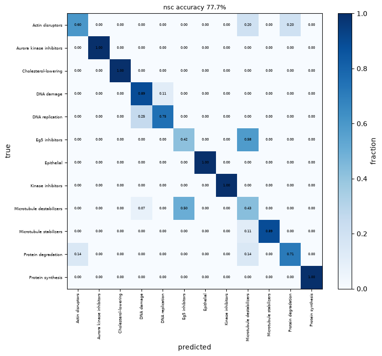
An off-diagonal block in the confusion matrix usually reflects biology.
ax = mt.pl.moa_confusion(signatures, key="nsc")
plt.show()
confusion = signatures.uns["mantispy"]["nsc_confusion"]
confusion[confusion["true"] != confusion["predicted"]].nlargest(5, "count")
| true | predicted | count | |
|---|---|---|---|
| 5 | Eg5 inhibitors | Microtubule destabilizers | 7 |
| 6 | Microtubule destabilizers | Eg5 inhibitors | 7 |
| 14 | DNA replication | DNA damage | 2 |
| 15 | Protein degradation | Actin disruptors | 1 |
| 16 | Protein degradation | Microtubule destabilizers | 1 |
The largest confusion is symmetric and biologically expected: Eg5 inhibitors and microtubule destabilizers, seven treatments each way. Eg5 is the kinesin that separates the centrosomes. Inhibiting it gives a monopolar spindle, and destabilizing microtubules also arrests mitosis. At these doses the two look alike under the microscope, which is a limit of the assay rather than of the classifier.
The second is DNA damage against DNA replication, for the same reason: both stall the cell cycle and both are read out through the DNA channel.
Which measurements separate the mechanisms#
var already records which object, measurement family and channel each feature belongs
to. tl.feature_sets turns that into a decoupler network, and tl.enrich scores every
signature against every set, so the result says which kinds of measurement moved instead of
which individual features.
BBBC021’s three channels are DAPI, tubulin and actin. The feature names spell them
CorrDAPI, CorrTub and CorrActin (the Corr prefix marks CellProfiler’s
illumination-corrected image, and the parser keeps the names as they are), and the table
below uses those names. If the enrichment carries signal, the tubulin-directed mechanisms
should load on the tubulin channel.
mt.tl.enrich(signatures, by="group_by_channel", method="ulm", tmin=5)
mt.tl.rank_sets(signatures, groupby="Metadata_MOA")

ranked = signatures.uns["mantispy"]["rank_sets"]
top = (
    ranked.sort_values("score", ascending=False)
    .groupby("group", observed=True)
    .head(2)
    .sort_values(["group", "score"], ascending=[True, False])
)
top.round(2)
| group | set | score | |
|---|---|---|---|
| 56 | Actin disruptors | Intensity|CorrTub | 3.12 |
| 55 | Actin disruptors | Intensity|CorrDAPI | 1.67 |
| 7 | Aurora kinase inhibitors | Intensity|CorrDAPI | 0.96 |
| 10 | Aurora kinase inhibitors | Texture|CorrDAPI | 0.11 |
| 69 | Cholesterol-lowering | Texture|CorrActin | 3.04 |
| 70 | Cholesterol-lowering | Texture|CorrDAPI | 2.99 |
| 46 | DNA damage | Texture|CorrDAPI | 0.10 |
| 47 | DNA damage | Texture|CorrTub | -0.51 |
| 41 | DNA replication | Texture|CorrTub | 0.78 |
| 40 | DNA replication | Texture|CorrDAPI | -1.14 |
| 12 | Eg5 inhibitors | Intensity|CorrActin | 3.84 |
| 14 | Eg5 inhibitors | Intensity|CorrTub | 1.65 |
| 22 | Epithelial | Texture|CorrDAPI | 1.29 |
| 23 | Epithelial | Texture|CorrTub | 0.83 |
| 29 | Kinase inhibitors | Texture|CorrTub | 1.18 |
| 28 | Kinase inhibitors | Texture|CorrDAPI | 1.11 |
| 48 | Microtubule destabilizers | Intensity|CorrActin | 3.13 |
| 51 | Microtubule destabilizers | Texture|CorrActin | 0.76 |
| 62 | Microtubule stabilizers | Intensity|CorrTub | 3.10 |
| 60 | Microtubule stabilizers | Intensity|CorrActin | 0.40 |
| 2 | Protein degradation | Intensity|CorrTub | 2.84 |
| 0 | Protein degradation | Intensity|CorrActin | 0.59 |
| 32 | Protein synthesis | Intensity|CorrTub | 4.47 |
| 31 | Protein synthesis | Intensity|CorrDAPI | 1.78 |
ax = mt.pl.sets_heatmap(signatures, groupby="Metadata_MOA", top=20)
plt.show()
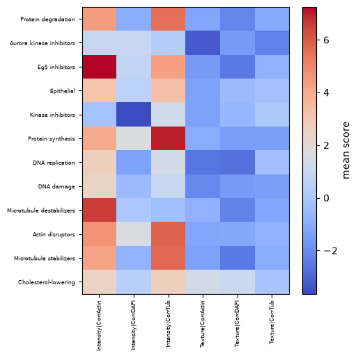
Microtubule stabilizers load most strongly on tubulin intensity. The pipeline was never told which channel stains microtubules; the channel comes from parsing the feature names, as in tutorial 1. This result therefore also checks the annotation.
The mapping is not one-to-one. Actin disruptors also score highest on tubulin intensity, and Eg5 inhibitors on actin. The two cytoskeletal systems are mechanically coupled, and a cell whose actin has collapsed looks different in every channel. Read the enrichment as which measurements changed, not as which protein was targeted.
Distances between mechanisms#
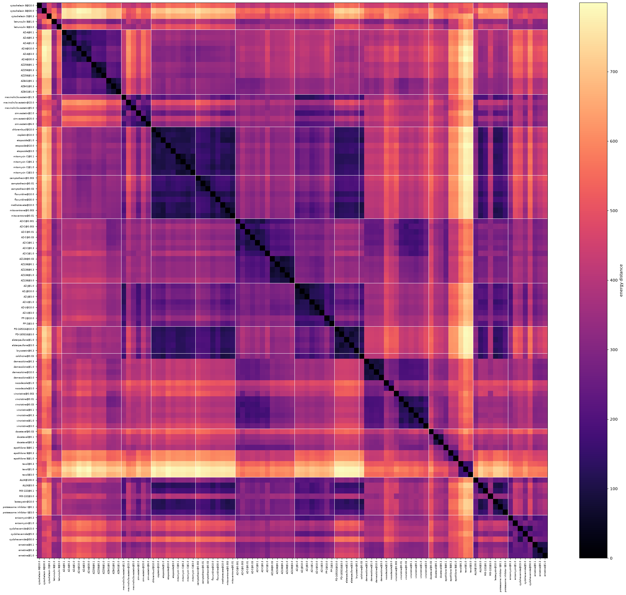
tl.edistance with reference=None gives the full treatment-by-treatment energy
distance matrix, and pl.distance_heatmap orders it by mechanism so related treatments sit
together.
mt.tl.edistance(signatures, reference=None)
ax = mt.pl.distance_heatmap(signatures, groupby="Metadata_MOA")
plt.show()
Scoring the whole map in one number#
The heatmap shows the mechanism blocks. metrics.known_relationships scores them: of the
compound pairs the annotation relates, what share lands in either tail of the map’s own
similarity distribution over all pairs? It is the benchmark Celik et al. [2024] selects
perturbative maps by, and it needs only an annotation of which perturbations belong together,
so the same call works for mechanisms here and for gene sets in a genetic screen.
Both tails count. Two compounds with opposite effects on one process are as related as two with the same effect, and a one-sided test would score an inhibitor and an activator of the same pathway as unrelated.
The profiles are aggregated to one per compound rather than one per treatment, so every annotated pair is two different molecules. That is the not-same-compound rule from the top of this page, applied to the annotation instead of to the classifier.
per_compound = treated.copy()
per_compound.obs["Metadata_Perturbation"] = per_compound.obs["Metadata_Compound"].astype(str)
compounds = mt.tl.consensus(per_compound, method="median", min_replicates=1)
compounds = compounds[compounds.obs["Metadata_MOA"].notna().to_numpy()].copy()

# source names a set, target one of its members. A mechanism is a set of compounds.
net = pd.DataFrame(
    {
        "source": compounds.obs["Metadata_MOA"].astype(str).to_numpy(),
        "target": compounds.obs["Metadata_Perturbation"].astype(str).to_numpy(),
    }
)

sizes = net["source"].value_counts()
{
    "compounds": int(compounds.n_obs),
    "mechanisms": int(sizes.size),
    "pairs sharing a mechanism": int((sizes * (sizes - 1) // 2).sum()),
    "pairs in total": compounds.n_obs * (compounds.n_obs - 1) // 2,
}
{'compounds': 38,
 'mechanisms': 12,
 'pairs sharing a mechanism': 44,
 'pairs in total': 703}
44 annotated pairs out of 703. A map that carried no information would put twice the tail size of them in the tails, so the baseline is known in advance rather than fitted. Shuffling the mechanism labels gives the same baseline empirically, which is the check that the statistic is calibrated on this map and not merely on paper.
generator = np.random.default_rng(0)
rows = []
for percentile in (1.0, 5.0, 10.0):
    observed = mt.metrics.known_relationships(compounds, net, percentile=percentile)
    shuffled = [
        mt.metrics.known_relationships(
            compounds,
            net.assign(source=generator.permutation(net["source"].to_numpy())),
            percentile=percentile,
        )["value"].iloc[0]
        for _ in range(20)
    ]
    rows.append(
        {
            "tail width (%)": percentile,
            "baseline": 2 * percentile / 100,
            "shuffled labels": float(np.mean(shuffled)),
            "observed": float(observed["value"].iloc[0]),
        }
    )

pd.DataFrame(rows).round(3)
| tail width (%) | baseline | shuffled labels | observed | |
|---|---|---|---|---|
| 0 | 1.0 | 0.02 | 0.016 | 0.136 |
| 1 | 5.0 | 0.10 | 0.105 | 0.500 |
| 2 | 10.0 | 0.20 | 0.201 | 0.659 |
The shuffled column sits on the baseline at all three widths, so the number means what it claims to. Against it, the observed recall is five times chance at the default width and close to seven times at the strictest one.
Read this next to the not-same-compound accuracy of 0.78 from the top of the page. They measure different things: the classifier asks whether the nearest neighbor of a compound shares its mechanism, while this asks how many of the annotated pairs are extreme in the whole distribution, including the pairs that are related but not nearest. The second is the harder question, and the smaller number is not a worse result.
values = np.asarray(compounds.X, dtype=float)
unit = values / np.linalg.norm(values, axis=1, keepdims=True)
similarity = unit @ unit.T

upper = np.triu_indices(compounds.n_obs, 1)
position = {name: index for index, name in enumerate(net["target"])}
related = [
    (position[a], position[b])
    for _, block in net.groupby("source")
    for index, a in enumerate(block["target"])
    for b in list(block["target"])[index + 1 :]
]

background = similarity[upper]
annotated = np.array([similarity[i, j] for i, j in related])
low, high = np.quantile(background, [0.05, 0.95], method="inverted_cdf")

fig, ax = plt.subplots(figsize=(6.5, 3.5))
ax.hist(background, bins=40, density=True, color="lightgrey", label=f"all {background.size} pairs")
ax.hist(
    annotated,
    bins=40,
    density=True,
    histtype="step",
    lw=1.8,
    color="seagreen",
    label=f"{annotated.size} sharing a mechanism",
)
for cut in (low, high):
    ax.axvline(cut, color="grey", ls="--", lw=1)
ax.set_xlabel("cosine similarity")
ax.set_ylabel("density")
ax.legend(fontsize=8)
plt.show()

{
    "annotated in the upper tail": int((annotated >= high).sum()),
    "annotated in the lower tail": int((annotated <= low).sum()),
}
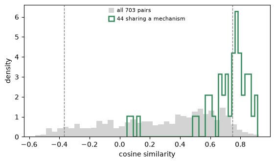
{'annotated in the upper tail': 23, 'annotated in the lower tail': 0}
The annotated pairs are shifted right of the background and pile up past the upper cut. None of them reach the lower one: at this granularity sharing a mechanism means looking alike, not looking opposed. The lower tail earns its place in genetic screens, where an activator and an inhibitor of one pathway are annotated together, rather than in a compound panel like this.
Per mechanism, the same statistic says which classes the assay resolves. Each row is scored against the same all-pairs background, so the rows are comparable.
per_mechanism = pd.DataFrame(
    [
        {
            "mechanism": mechanism,
            "compounds": len(block),
            "pairs": len(block) * (len(block) - 1) // 2,
            "recall": mt.metrics.known_relationships(compounds, block)["value"].iloc[0],
        }
        for mechanism, block in net.groupby("source")
        if len(block) > 1
    ]
)
per_mechanism.sort_values("recall", ascending=False).round(3)
| mechanism | compounds | pairs | recall | |
|---|---|---|---|---|
| 1 | Aurora kinase inhibitors | 3 | 3 | 1.000 |
| 2 | Cholesterol-lowering | 2 | 1 | 1.000 |
| 5 | Eg5 inhibitors | 2 | 1 | 1.000 |
| 9 | Microtubule stabilizers | 3 | 3 | 1.000 |
| 11 | Protein synthesis | 3 | 3 | 1.000 |
| 3 | DNA damage | 4 | 6 | 0.667 |
| 8 | Microtubule destabilizers | 4 | 6 | 0.500 |
| 0 | Actin disruptors | 3 | 3 | 0.333 |
| 4 | DNA replication | 4 | 6 | 0.333 |
| 6 | Epithelial | 3 | 3 | 0.333 |
| 7 | Kinase inhibitors | 3 | 3 | 0.000 |
| 10 | Protein degradation | 4 | 6 | 0.000 |
Five mechanisms recover every pair: Aurora kinase inhibitors, Eg5 inhibitors, microtubule stabilizers, protein synthesis inhibitors and the two cholesterol-lowering compounds. These are the classes with one clear cellular readout.
Two recover none, and both were already flagged earlier on this page by a different method. Protein degradation is the class where ALLN, MG-132 and lactacystin each drew a different wrong answer in the blind test above; here their profiles are not even mutually extreme, which is the same finding with no classifier in the way. Kinase inhibitors is a label covering different kinases with different substrates, so there is no reason for its members to converge on one morphology — the annotation is broad, not the assay blind.
That distinction is the point of reading the per-mechanism table rather than the single number. A low overall recall can mean the map is poor, or it can mean the annotation groups things the assay has no reason to group, and only the breakdown separates the two.
Summary#
Report the not-same-compound number, or state which rule you used. The gap between the two is large enough to change conclusions.
Chance is the largest class’s share, not one over the number of classes.
Confusions are hypotheses about the assay. The confusion between Eg5 inhibitors and microtubule destabilizers shows what these images can resolve.
metrics.known_relationshipsscores the whole map against an annotation in one number, read against a baseline of twice the tail width. The per-mechanism breakdown says whether a low number is the map or the annotation.moa_enrichmentscores a compound without a label, as needed in a screen of uncharacterized molecules.
Next: single-cell heterogeneity, on what a well median hides.